Hopf fibration
Produced using manim.
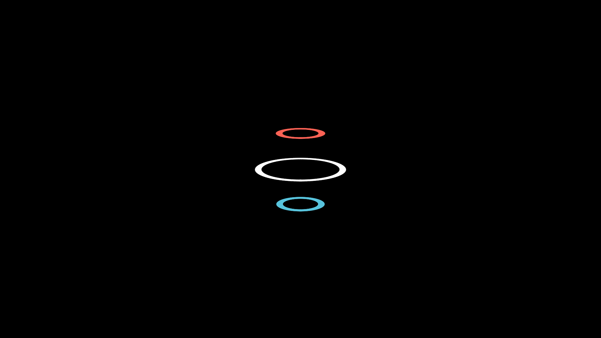
Consider three circles of constant z on S2. Under the Hopf map, the preimage of each point is a circle in S3. Then we might expect the preimage of a circle of points to be a (potentially distorted) torus. We can pick some nice charts of the 3-sphere so that these preimages look nice.
This is their preimage under stereographic projection, (w, x, y, z) ↦ (x,y,z)/(1-w).
This is their preimage under the two balls view, (w, x, y, z) ↦ (x, y, 2×sign(w) + z).
This is their preimage after projecting onto SO(3). (w, x, y, z) ↦ w + xi + yj + zk as a quaternion, which can then be identified with an SO(3) matrix by conjugating pure quaternions.
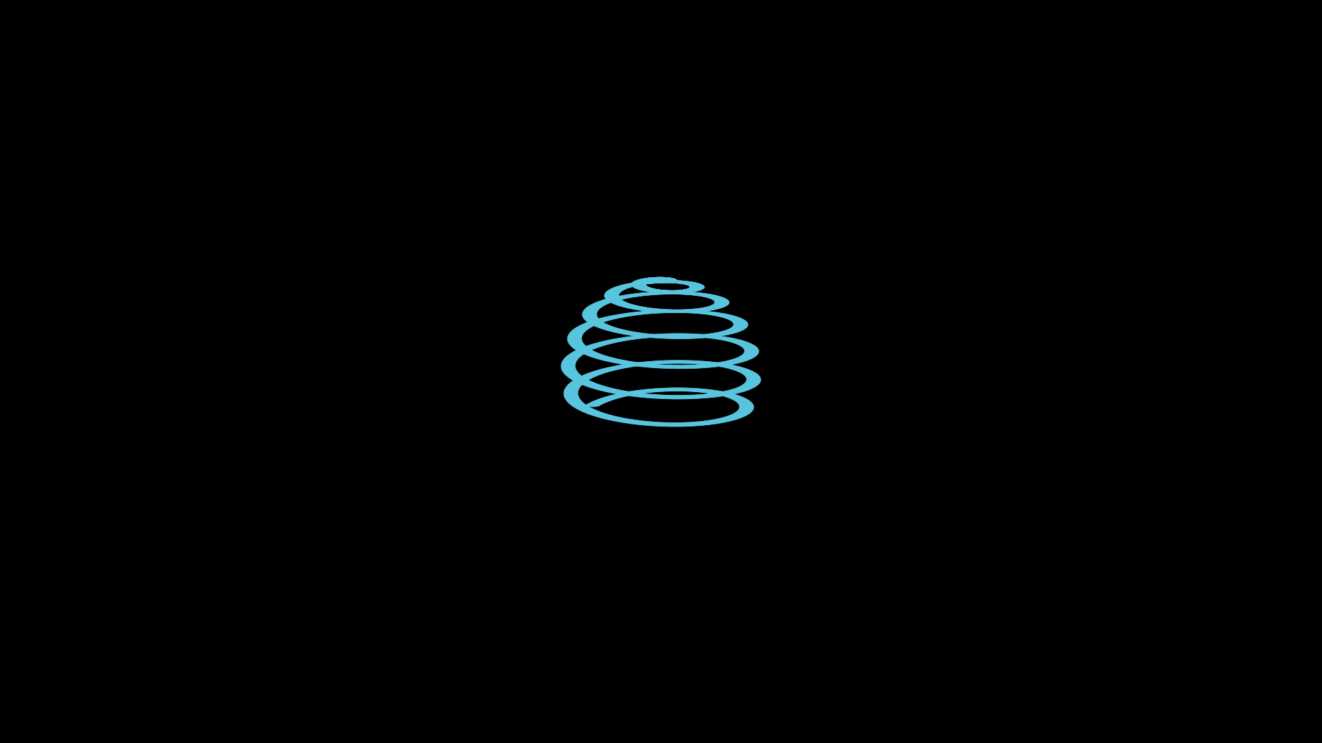

The animation on the right is the preimage of the spiral on the left, going down the spiral. As the spiral on S2 becomes denser and fills out the sphere, so too will the toroidal spiral on the right fill out R3.
A Youtube video again visualising the Hopf map using stereographic projection, with cool music. too.
Hopf fibration as a principal U(1) bundle
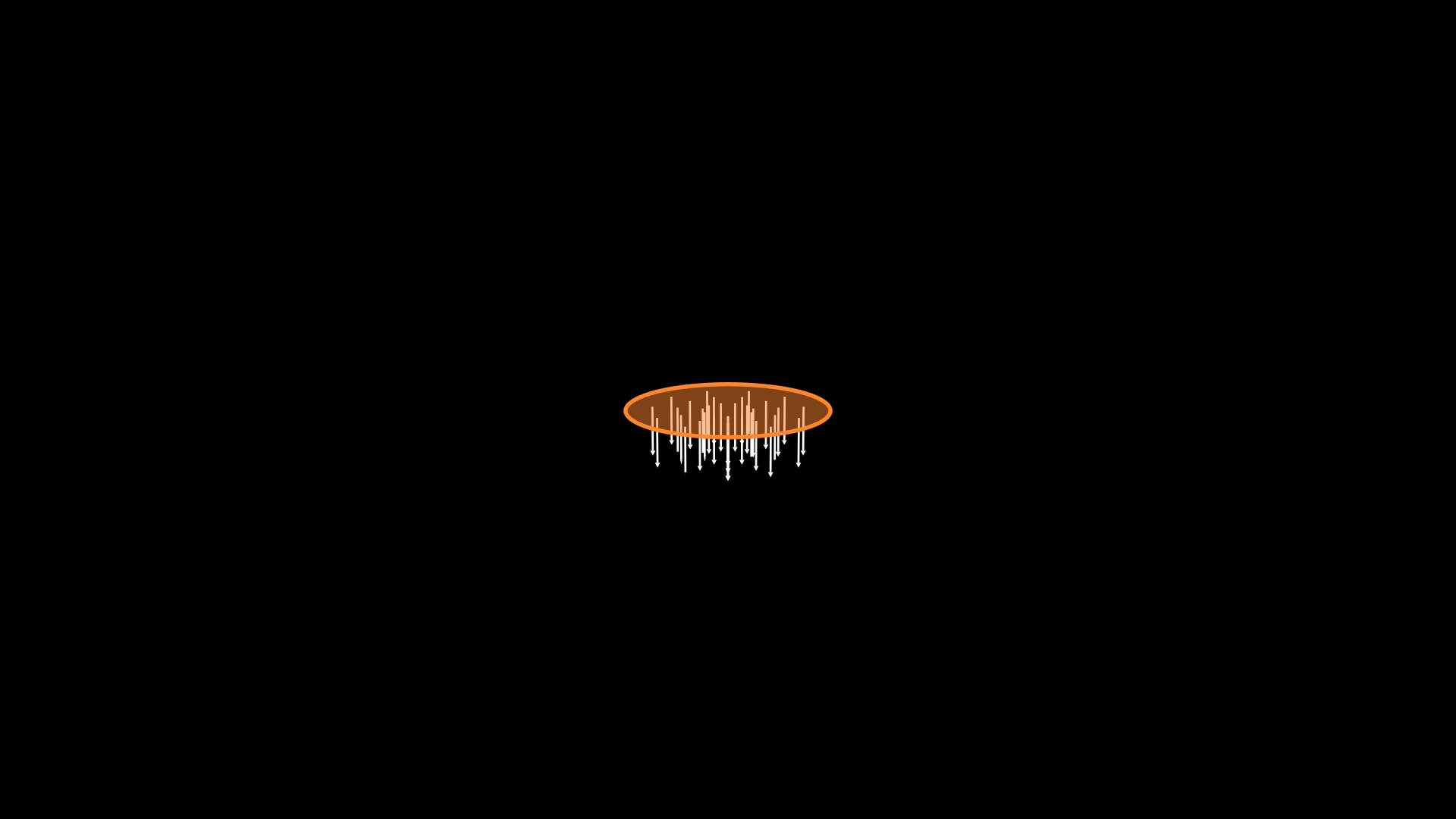
Work under stereographic projection. Each point on the sphere corresponds to a Villarceau circle on these tori of constant height. Each of these circles intersects with the unit disc on the z=0 plane (without boundary) exactly once, except for the circle corresponding to the south pole, which forms the boundary of the unit disc. Then we pick a (cross) section by mapping each circle to the corresponding point on the unit disc. This corresponds to a trivialisation over S2 minus the North pole, as it picks a 'base point' for each of these circles, turning them into U(1) with identity at the base. The section is shown as an orange disc on the gif.
After picking this trivialisation we can see a U(1) action on S3, shown by the action on a selection of points shown in white. The points flow along the fundamental vector field for the Hopf bundle.
We can come up with new trivialisations over the same subset of the base using (smooth) functions α:S2 ↦ R, since eiα is a function to U(1). Then we get a new section by flowing each point on the disk by eiα around its associated circle.
This is related to gauge transformations in physics. Given a gauge field (in physics language) or a connection (in mathematical language), the gauge transformation sends our gauge field A ↦ A + dα, which is exactly how the connection transforms under change of trivialisation.
What does a (principal) connection look like?
This may sound like nonsense, but let me propose what it looks like, and then I'll justify it. Under stereographic projection, we can visualise a (principal) connection on this bundle via a (smooth) assignment of vectors (which have WLOG unit length) to R3 which is nowhere perpendicular to the fundamental vector field, with certain consistency requirements for vectors on the same orbit.
On principal bundles there is an identification between elements of the Lie algebra and fundamental vector fields on the bundle, which generate flow along the part of the bundle that looks like a Lie group.
We use that in R3, vectors correspond to a single plane to which they are normal. By considering projective vectors, where two nonzero vectors which differ by a nonzero scalar are the same, this correspondence is bijection. Using this notion of orthogonality is sort of cheating; it uses the geometry of this chart, stereographic projection, not the geometry of S3.
These planes give an assignment of horizontal subspaces to each point of S3, in other words, a horizontal distribution. These subspaces are the kernel of the principal connection at each point. The principal connection is a 1-form. We can think of the connection as defining a projection of vectors onto the fundamental vector field.
In the tangent space at p, there is a line in the tangent space corresponding to the fundamental vector field, and another line corresponding to the connection, not orthogonal to the fundamental vector field line. Given a vector, in the tangent space, we can slide the head of the arrow in a plane orthogonal to the connection line, until we hit the fundamental vector field line. This construction ensures that the fundamental vector field is unchanged, so this really is a projection onto the fundamental vector field.
Explicitly, restrict to a single tangent space at p, let n be the connection normal vector at p, ξ be the fundamental vector field at p. Then v ↦ Pv = (v·n)ξ/(v·ξ).
To ensure the connection is compatible with the bundle structure, there is also a requirement of right equivariance, which tells us how to relate horizontal subspaces on different points of the orbit. So it is enough to just specify the horizontal subspace on one point of each orbit. So here's a connection, defined on most of the bundle, with the vector just pointing downward on each point of the unit disc.
Right equivariance

The gif shows how to determine the connection at other points on the same orbit. We take the normal plane to the vector in R3 to get the horizontal distribution at p, H(p). We then take two vectors spanning H(p), and parallelly transport them (using Lie derivative) along the U(1) orbit, defining a horizontal subspace at H(p·g). Then again take the normal vector in R3 to get the 'connection vector' at p·g. Again, be warned that the 'connection vector' relies on the geometry of the projection, not of S3. And full disclosure: I haven't done the calculation to parallelly transport the vectors in this particular gif, but it is possible to find a nice form for how vectors transform by solving the parallel transport equation, which I'll leave to you.
This shows the notion of right equivariance for principal bundles. In some sense, the connection must be 'blind' to where along the fibre you are evaluating it.
Projection

The purple vector is a vector v on the principal bundle which we input into the principal connection 1-form. The horizontal distribution H evaluated at p tells us how to assign an element of the Lie algebra to the vector.