Manim animations
Joukowsky transform
The Joukowsky map f(z) = z + 1/z applied to a circle of radius 1.08, centred at (-0.08, 0.08).
Torus twist
Dehn twist or something, I'm not a geometer.
Left Invariant Vector Fields

This probably deserves its own page. If you can't be bothered to read through the text below (which is entirely justified), skip to the bottom for another animation and a picture showing the vector field in more detail.
On a smooth (Lie) group, the left invariant vector fields are vector fields which don't change after being pushed forward by any element of the group. Under the vector field commutator, these vector fields form a Lie algebra: the Lie algebra of a Lie group, or following my own descriptive convention: the infinitesimal algebra of a smooth group. What does a left invariant vector field look like?
The top case is the U(1) case, with some arrows representing the unique (up to rescaling) left invariant vector field. The vector field is being pushed forward by rotations of π/3. It's not very interesting, but serves as a useful warmup for thinking about what is happening. Note here a possible point of confusion: the vector field is not flowing along itself, but being pushed forward by the left-translation diffeomorphism.
The bottom case is the SO(3) vector field representing infinitesimal rotations in the z-direction. The animation makes use of maps between SO(3), its matrix Lie algebra so(3), and vectors in R3, and ultimately it is the ability to identify elements of SO(3) and so(3) with 3D vectors that allows us to see the vector field. This is much more interesting as it is a non-abelian Lie group. It sits in somewhat of a sweet spot as it is not trivial like U(1), but is low dimensional enough (i.e. has real dimension < 4) that it can be visualised.
What is meant by the 'matrix Lie algebra' of a Lie algebra? If G is a matrix Lie group, then its tangent space at the identity can be identified with a linear space of matrices, and spaces of matrices have an existing product from which a commutator can be constructed. There is a bijection between left-invariant vector fields and the tangent space at any point of G, and in particular at the identity. This bijection is linear, and after equipping each space with its commutator, an isomorphism of algebras. Next we discuss these maps.
There is a linear isomorphism between vectors in R3 and so(3), which can be identified with antisymmetric matrices. The map to so(3) comes from contracting the vector with the totally antisymmetric Levi-Civita epsilon. The inverse comes from contracting the matrix on both indices with the epsilon, up to a factor which you can determine yourself.
I like to think of the map R3 to so(3) in the following way though: the cross product of two vectors u×v is linear in v, so we can see the partial evaluation of the cross product 'u×' as a linear map. Then u↦u× is the required map. I like thinking about partial evaluations of maps, and may do a page on them.
From an so(3) matrix, we get an SO(3) matrix via matrix exponentiation. From an SO(3) matrix, we get a vector via the axis-angle map. If R∈SO(3) is a rotation by θ about a normalised axis n, then R↦θn, and this is an inverse to the matrix exponentiation after identifying R3 and so(3). But θ is not unique. To ensure we get a unique inverse, we restrict θ to the range [0, π]. This is a choice of a branch of logarithm for the exponential map.
Now, an explanation of what the animation shows. The points on the filled ball are elements of SO(3) under the axis-angle map. Calling the vector field ξ, at each point R on the ball we assign a vector in the tangent space at that point ξ(R). This is achieved by pushing forward ξ(I), where I is the identity in SO(3), by the left-translation diffeomorphism LR. Since these are both matrices, we get ξ(R)=Rξ(I). We can't immediately associate a vector to this matrix, but we can if we apply R-1 to the other side. Calling the map from so(3) → R3 T, the 3D vector is v(R) = T(ξ(R)R-1).
Left invariance means that after pushing forward the vector field by any element of the group, the vector field will be unchanged. For these animations, this means that if we have an assignment of arrows to each point (here we can only do a finite selection), then after each pushforward we get back the same assignment of arrows.
Note, when the arrows move from the top of the sphere to the bottom, ideally the arrows would continue upward through the boundary of the sphere and reappear at the bottom via the identification of antipodal points, but I haven't yet figured out how best to animate this :(.
The vector field must be invariant after pushing by any rotation. Here it is being pushed forward by rotations about the x-axis.
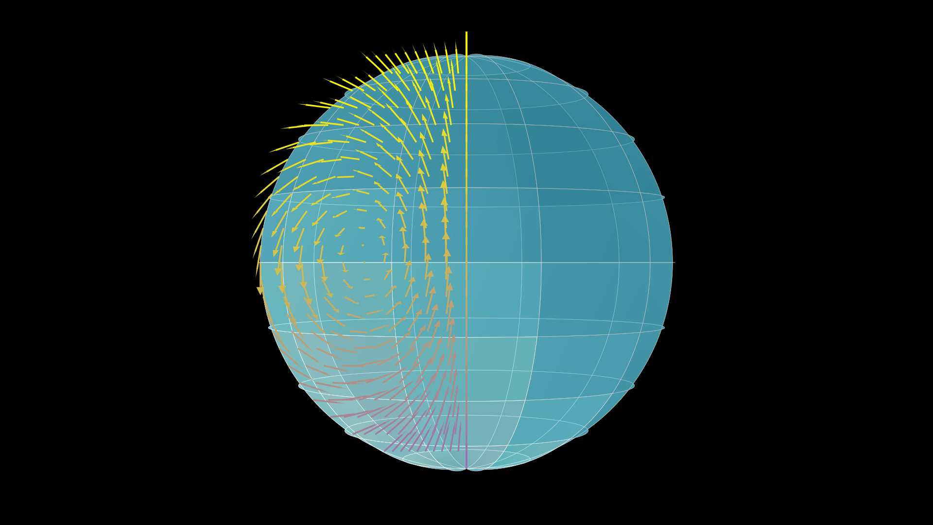
And here is the vector field, plotted on a half plane y = 0, x > 0. This is all that's needed to get a general picture due to axisymmetry of the vector field. You'll need to deduce whether the arrows point into or out of the y = 0 plane from the animations, by conjugating, or by thinking about what a tiny rotation about z looks like from the point of view of someone who sees the sphere rotated by R relative to you.