Root systems
Introduction
The classification of (finite, irreducible) root systems is that there are four countably infinite families, and five exceptional root systems.
The countably infinite families are labelled \(A_n, B_n, C_n\) and \(D_n\) for \(n \in \mathbb{Z}_{>0}\). The exceptional systems are \(G_2, F_4, E_6, E_7\) and \(E_8\).
The subscript denotes the dimension of the space \(\mathbb{R}^n\) that the root system lives in. At its simplest, a root system is a finite set of \(n\)-vectors satisfying certain reflection properties.
The four families \(A_n, B_n, C_n, D_n\)
Input a type (out of \(A, B, C\) or \(D\)) and the rank \(n\). Note \(D_2\) does not work, but is easily visualizable as it is \(A_1\times A_1\). This generates the projection of the root system onto the Coxeter plane.
Root systems of low dimension
The root systems of dimension 2 can be straightforwardly visualized. The root systems of dimension 3 can be visualized. For higher dimension, the root system must be projected to a lower-dimensional subspace. It turns out there is a preferred plane, the Coxeter plane, to project any root system onto.
One-dimensional root system: \(A_1\)
Consists of the two points \(\pm 1\). Very boring, but the most important root system.
Two-dimensional root systems: \(A_2, B_2, G_2\)
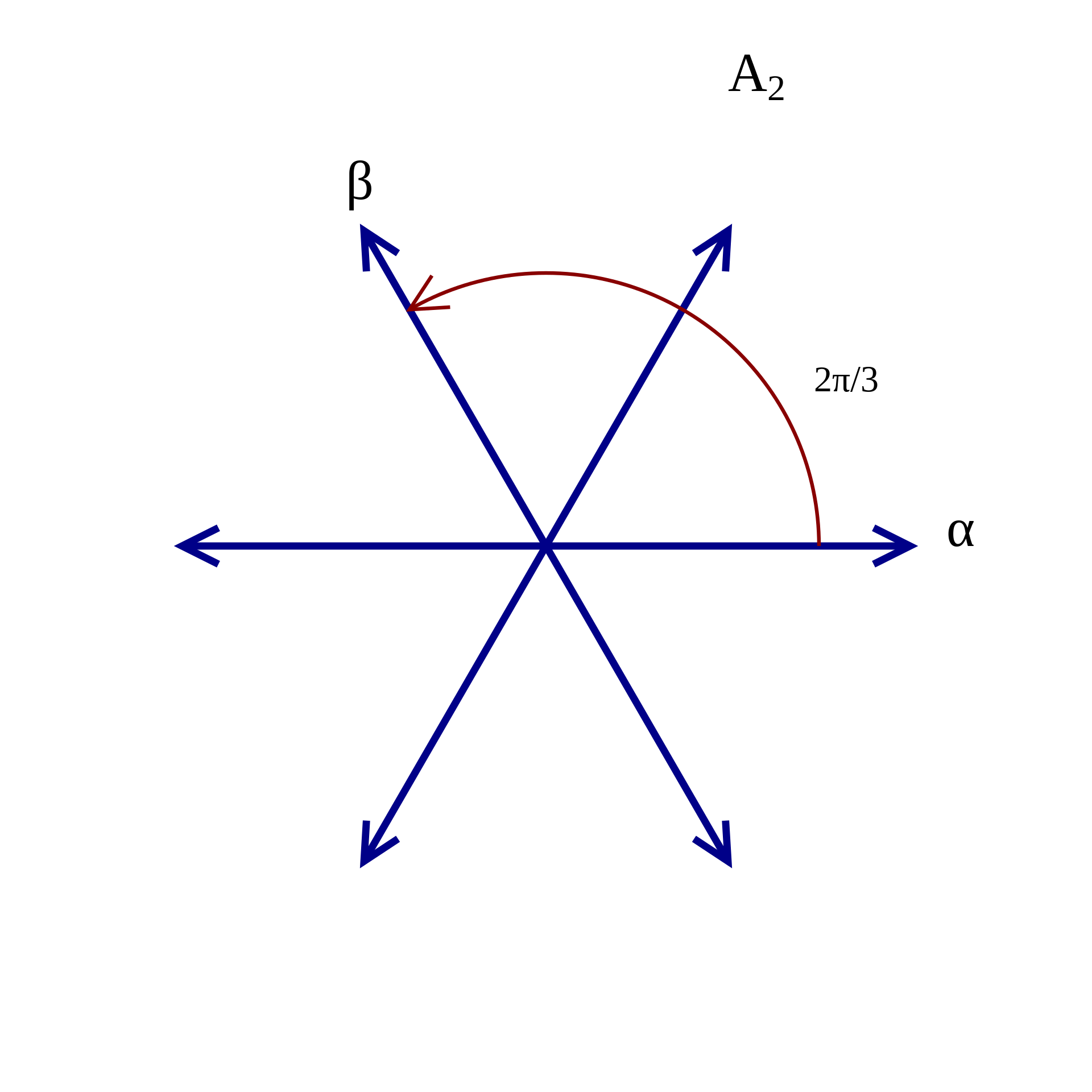
These are the three simple root systems of dimension 2. \(C_2\) is the same as \(B_2\), while \(D_2\) is not simple as it decomposes into two copies of \(A_1\).
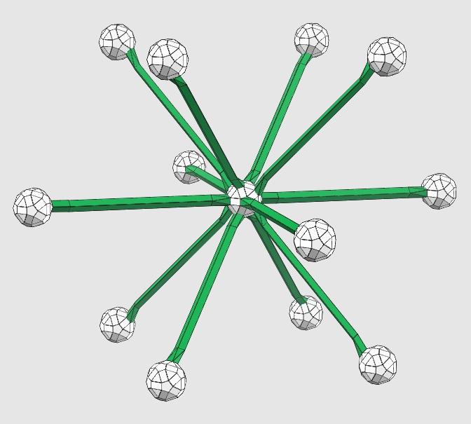
Three-dimensional root systems: \(A_3, B_3, C_3\)
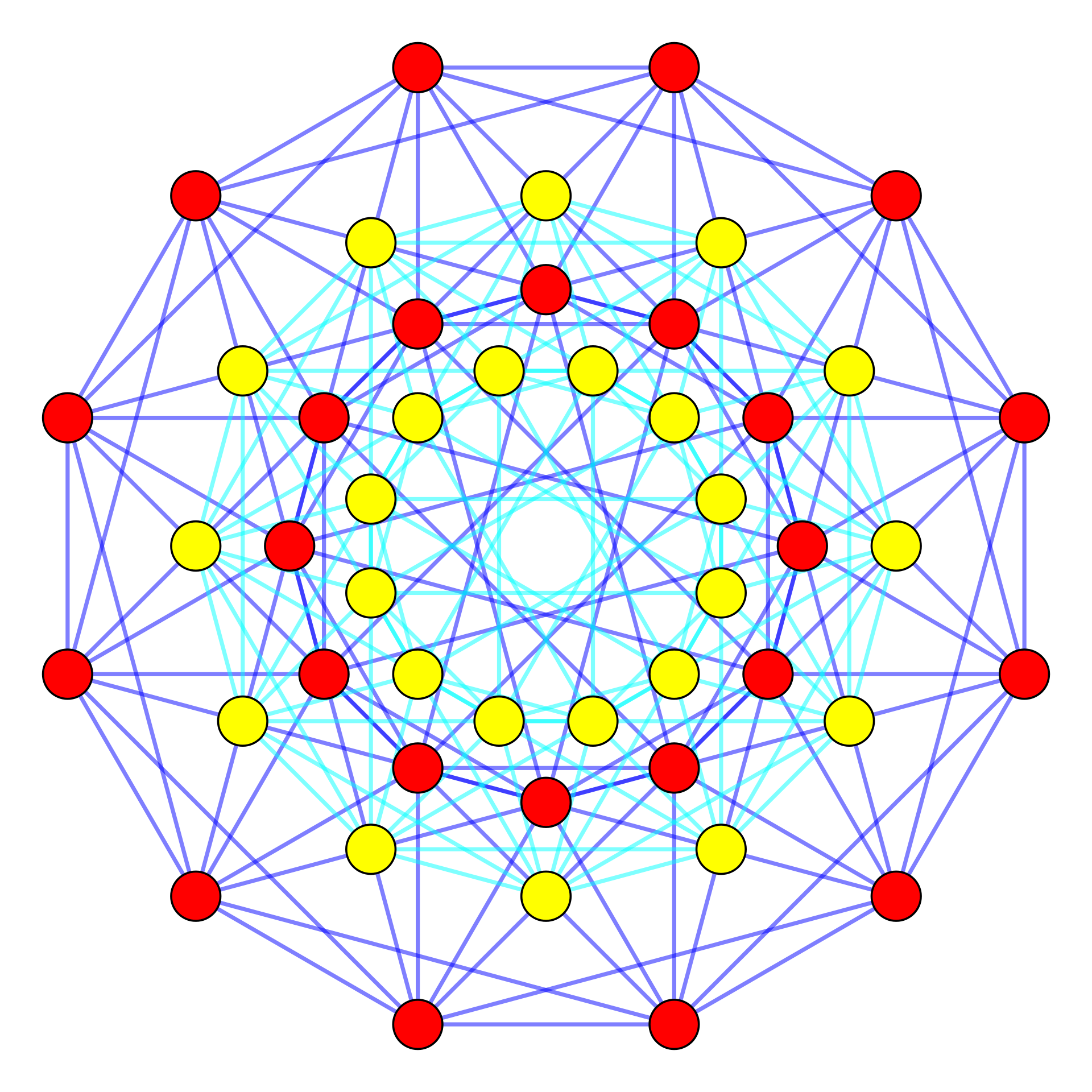
The other exceptional root systems: \(F_4, E_6, E_7, E_8\)
Coxeter plane projections
For \(E_6\), the orange vertices have multiplicity 2.
How are these generated?
The starting point is the root data and simple root data \(\Phi_s \subset \Phi \subset \mathbb{R}^n, |\Phi| < \infty\). This can be found online for the different root systems. For any vector \(v\) in \(\mathbb{R}^n\), there is a reflection map \[s_v: u \mapsto u - 2\frac{\langle u,v\rangle}{\langle v,v\rangle} v.\] The simple reflections are the reflections defined by the simple roots \(\alpha_i \in \Phi_s\). The Coxeter element is the* product of all the simple reflections taken in any order.
From Lie theory, the Coxeter element's eigenvalues are distinct phases. The Coxeter plane is the unique real plane on which the Coxeter element has complex eigenvalues \(e^{i\alpha}, e^{-i\alpha}\) with \(\alpha\) positive but minimal among the possible phases.
* There is not a unique way to take their product but it doesn't matter much which order is taken.
Attributions
\(A_2, B_2, G_2\): By User:Maksimderivative work: Smithers888 (talk) - Root-system-G2.png, CC BY-SA 3.0, https://commons.wikimedia.org/w/index.php?curid=8547784
\(A_3, B_3, C_3\): Lie Groups, Lie Algebras, and Representations: An Elementary Introduction by Brian C. Hall ISBN 9780387401225, produced using ZomeTool
\(F_4\): By Tomruen - Own work, Public Domain, https://commons.wikimedia.org/w/index.php?curid=12338859
\(E_6\): By User:Tomruen - Own work, Public Domain, https://commons.wikimedia.org/w/index.php?curid=12179922
\(E_7\): By Claudio Rocchini - Own work, CC BY 3.0, https://commons.wikimedia.org/w/index.php?curid=4744187
\(E_8\): By Jgmoxness - Own work, CC BY-SA 3.0, https://commons.wikimedia.org/w/index.php?curid=8893046