Pseudospheres and sine-Gordon Solitons
Introduction
Based an AMS article written by Chuu-Lian Terng and Karen Uhlenbeck, titled "Geometry of Solitons".
Pseudospheres (or pseudospherical surfaces), like spheres, are surfaces of constant curvature in \(\mathbb{R}^3\). Unlike spheres, they have constant negative curvature, that is, they are everywhere hyperbolic. There's a theorem due to Hilbert (which I would call the pseudosphere non-regularity theorem) which says any immersion of the pseudosphere cannot be regular. Nevertheless, one example of a pseudosphere, sometimes called the pseudosphere, fails to be regular in a pretty tame way: it is regular except for a cuspidal circle. Another name for the pseudosphere is the tractroid, as it is the volume of revolution from a parametric surface called the tractrix about its asymptote.
The sine-Gordon equation is a hyperbolic, nonlinear partial differential equation given by \[\varphi_{uv} = \sin\varphi\] or in different coordinates, \[\varphi_{xx} - \varphi_{tt} = \sin \varphi.\]
A remarkable amount is known about its solutions given that it is a nonlinear. It is Lorentz invariant, so for any solution \(\varphi(x,t)\), any boost is also a solution. More explicitly, \(\varphi(x\cosh\xi + t\sinh\xi, t\cosh\xi + x\sinh\xi)\) is also a solution for any real \(\xi\). So any solution is in fact part of a one-parameter family of solutions. But there are furthermore many of these families of solutions, to which we can associate integers such as the soliton number and the winding number.
The focus of this page is on a cute and unexpected correspondence between pseudospherical surfaces and solutions to the sine-Gordon equation.
The Simplest Case
The simplest case of the correspondence is between the tractroid on the pseudosphere side and the static one-soliton on the sine-Gordon side, so-called as it is independent of time: \(\varphi(x,t) = \varphi(x)\).
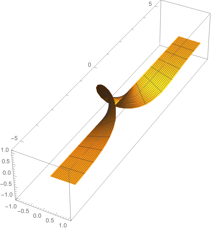
An explicit parametrisation for the tractrix is \[x(t) = t - \tanh(t), y(t) = \mathrm{sech}(t)\]
and so the tractroid, its volume of revolution, has parametrisation \[x(t,\theta) = \mathrm{sech}(t)\cos(\theta), y(t,\theta) = \mathrm{sech}(t)\sin(\theta), z(t,\theta) = t - \tanh(t).\]
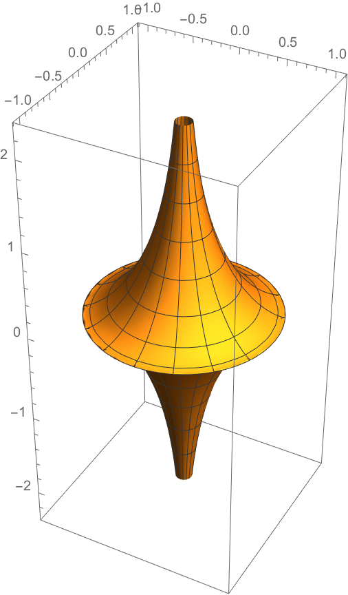
From these figures we see the tractroid fails to be regular only on a circle at \(z = 0, x^2 + y^2 = 1\). Ex: show the tractroid has constant Gauss curvature \(-1\) everywhere else.
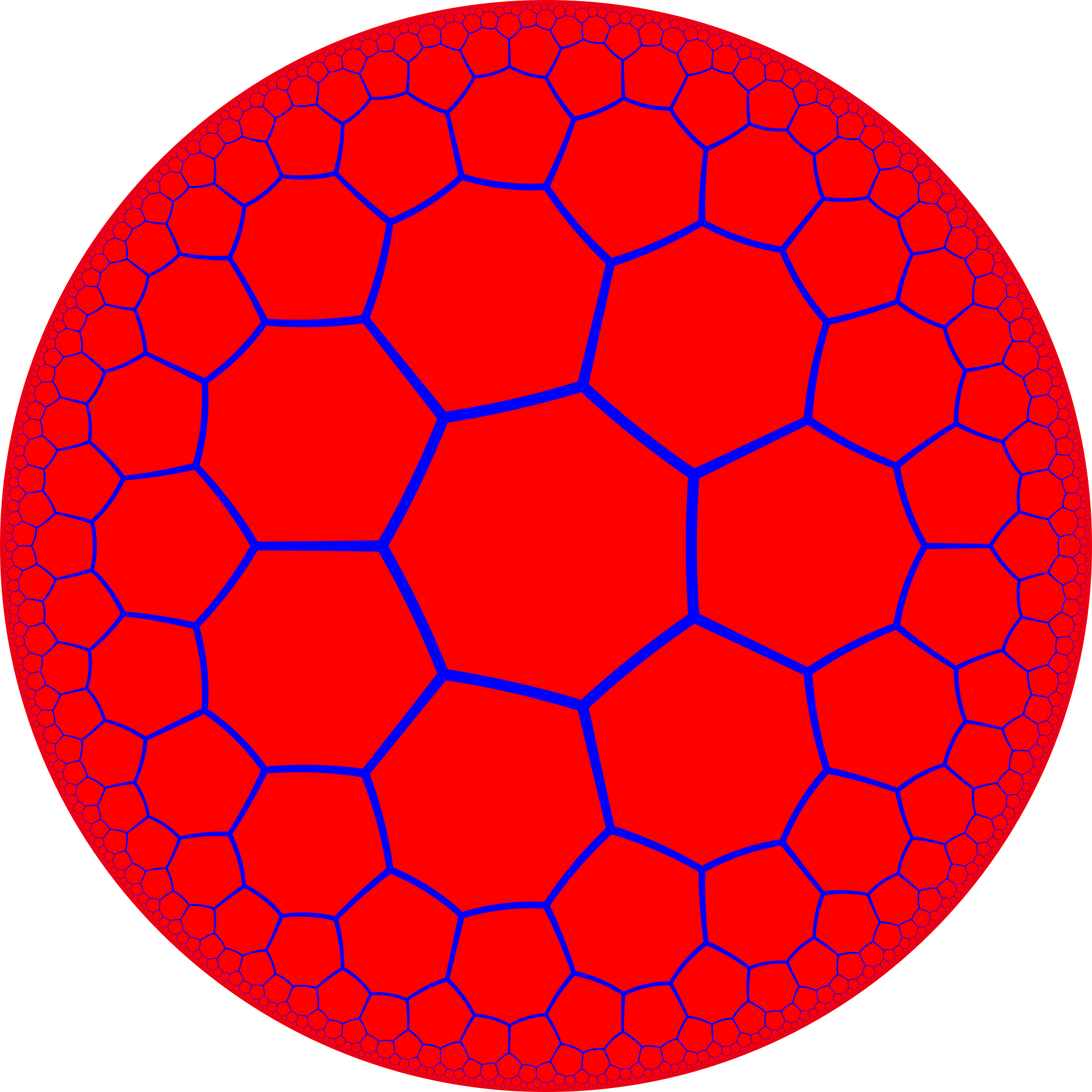
Spaces with everywhere constant negative curvature are called hyperbolic space. What distinguishes pseudospherical surfaces from other models of hyperbolic space are that they are "close" to immersions in \(\mathbb{R}^3\). While other models of hyperbolic space such as the half-plane or disc model are very nice to work with mathematically, they necessarily distort the metric, so it requires some mental gymnastics to visualize how distances work in these models. Visualization tricks such as tesselations are needed to get used to visualizing distances in these models.
By contrast, pseudospherical surfaces allow us to see hyperbolicity in our space, without distortion. There are examples of local hyperbolic curvature in our everyday life: for example at the centre of a pringle, or in many examples of the natural world such as leaves and corals, but these do not have everywhere constant curvature, so fail to be models of hyperbolic space. On the tractroid, we can see how the constant curvature is maintained: on this spindle shape, as we go spindle-ward, the radius gets smaller and hence the surface is more curved in the radial direction, but this is compensated by decreasing curvature in the z-direction as the asymptote is approached.
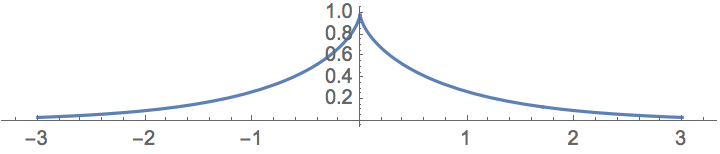
The static soliton is given by \[\varphi(x) = 4\arctan(e^x).\]
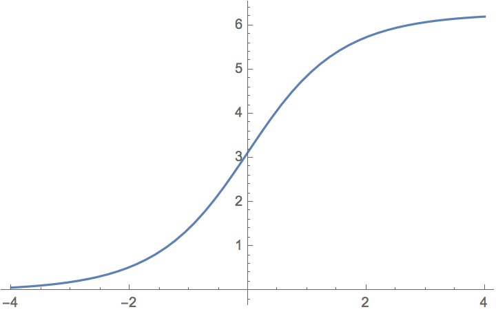
Ex: Check it is a solution to the static sine-Gordon equation, \(\varphi'' = \sin\varphi\). Another thing which tends to surprise me is how symmetric it is, considering its form, but it is less surprising upon considering \(\varphi(x) + \varphi(-x)\). We can also calculate the winding number for this solution: \[I[\varphi] = \frac{1}{2\pi}[\varphi(x,t)]^{+\infty}_{-\infty} = \frac{1}{2\pi}\left(\lim_{x \rightarrow +\infty}\varphi(x,t) - \lim_{x \rightarrow - \infty}\varphi(x,t)\right),\] which in this case is easily calculated to be \(1\).
There are several clues to suggest \(\varphi\) is better thought of as a phase, so that \( u = e^{i\varphi}\) is the more natural function to consider. Firstly there is this winding number. There is also the fact that if \(\varphi\) is a solution, so is \(\varphi + 2\pi\) and more generally \(\varphi + 2k\pi\). If you're familiar with variational principles, the sine-Gordon equation emerges as the equation of motion starting from the Lagrangian \[\mathcal{L} = u_xu^*_x - u_tu^*_t + \frac{u + u^*}{2}.\]
The Gauss–Codazzi equations and the correspondence
The maths behind the correspondence is mostly contained in the Gauss–Codazzi equations for embedded subsurfaces, which pseudospheres are by definition. We will only discuss the mathematics of the correspondence briefly as the visuals are the main focus.
Every embedded surface in \(\mathbb{R}^3\) has two associated two-by-two symmetric matrix valued functions called the first fundamental form \(I\) and second fundamental form \(II\), and in this setting the Gauss–Codazzi equations are a system of second order PDEs in the six components of the first and second fundamental forms.
The first fundamental form is also the induced metric which is the pull-back of the metric from \(\mathbb{R}^3\), so it is necessarily positive definite. Where the surface has negative Gauss curvature, with Gauss curvature \(K\) given by \[K = \frac{\mathrm{det}II}{\mathrm{det}I},\] necessarily we have \(\mathrm{det}II < 0\). Interpreting the second fundamental form as a bilinear form, it necessarily has signature \((+,-)\), and therefore has two independent 'null' directions \(u,v\) in the tangent space so that \(II(u,u) = II(v,v) = 0\). These can be used to define local asymptotic coordinates.
Pseudospherical surfaces further have a special set of asymptotic coordinates so that the fundamental forms can be put in the form \[I = \begin{pmatrix}1 & \cos\varphi \\ \cos\varphi & 1\end{pmatrix}, II = \begin{pmatrix}0 & \sin\varphi \\ \sin\varphi & 0\end{pmatrix},\] so that the Gauss–Codazzi equations reduce to the sine-Gordon equation in null coordinates, \(\varphi_{uv} = \sin\varphi\). This gives the pseudospherical surface → sine-Gordon solution direction. Given a parametrized pseudospherical surface, in theory we can switch to the preferred asymptotic coordinates then read off \(\varphi\) from the fundamental forms.
For the converse, the fundamental theorem of embedded surfaces states that for any pair of symmetric matrices obeying the Gauss–Codazzi equations are the first and second fundamental forms of some maximal embedded surface, unique up to rigid motions. But then since matrices of the form given above satisfy the Gauss–Codazzi equations so long as \(\varphi\) is a solution to the sine-Gordon equation, the theorem provides a way to construct surfaces, and it is easily verified these are pseudospherical.
There's a nice physical interpretation of the Gauss–Codazzi equations in terms of elastic theory. An elastic membrane can be thought of as a surface with its own intrinsic metric, which is its rest shape. But it can be deformed so that the membrane is under tension, and it obtains an extrinsic metric from how it fits into three-dimensional space. The Gauss–Codazzi equations are then compatibility conditions for when the elastic membrane is at rest, that is, it is not under tension due to deformation.
One-Parameter Family
Earlier, we mentioned that for any solution to the sine-Gordon equations, there's a one-parameter family of solutions given by boosts. Applied to the static soliton, we obtain a family parametrized by \(\xi\) giving the solutions \[\varphi_\xi(x,t) = 4\mathrm{arctan}(e^{x\cosh\xi + t\sinh\xi}).\] These give moving one-solitons with rapidity \(\xi\). For example, choosing \(\xi = -\log(2)\) gives \[\varphi_{-\log(2)}(x,t) = 4\mathrm{arctan}(e^{5x/4 - 3t/4}),\] moving at velocity \(v = + 3/5\).
On the pseudosphere side of the correspondence, there must be a one-parameter family of pseudospheres, which further can come from deformations of the standard pseudosphere. These are known as Dini's surfaces.